How many CPU cores can you actually use in parallel?
When you’re running a CPU-intensive parallel program, you often want to have a thread or process pool sized by the number of CPU cores on your machine. Fewer threads and you’re not taking advantage of all the cores, more than that and your program will start running slower as multiple threads compete for the same core. Or that’s the theory, anyway.
So how do you check how many cores your computer has? And is this actually good advice?
It turns out to be surprisingly tricky to nail down how many threads to run:
- The Python standard library provides multiple APIs to get this info, but none are sufficient.
- Even worse, because of CPU features like instruction-level parallelism and simultaneous threading (aka Hyper-threading on Intel CPUs), the number of cores you can effectively use depends on the code you have written!
Let’s see why it’s so difficult to figure out how many CPU cores your program can use, and then consider a potential solution.
Getting the number of CPU cores from Python
If you read the Python standard library documentation, it has a os.cpu_count() function that returns “the number of logical CPUs in the system”.
What does logical mean?
We’ll get to that in a bit.
The documentation also tells you that “len(os.sched_getaffinity(0)) gets the number of logical CPUs the calling thread of the current process is restricted to”.
Scheduler affinity is a way to restrict a process to particular cores.
Unfortunately, this API is not sufficient either.
For example, on Linux the cgroups API, used to implement Docker and other container systems, has a variety of ways to limit CPU usage.
Here we limit the CPU to the equivalent of 2.25 cores; the mechanism is different, but the effects will be similar:
$ docker run -i -t --cpus=2.25 python:3.12-slim
Python 3.12.1 (main, Dec  9 2023, 00:21:37) [GCC 12.2.0] on linux
Type "help", "copyright", "credits" or "license" for more information.
>>> import os
>>> os.cpu_count()
20
>>> len(os.sched_getaffinity(0))
20
We can only use the equivalent of 2.25 cores at a time, but neither API knows about this.
What’s a logical CPU?
Operating system options are just the start of our troubles, but before we see an example we need to understand what physical and logical CPU cores are. My computer use an Intel i7-12700K processor, which has:
- 12 physical cores (8 performance cores, and 4 less powerful ones).
- 20 logical cores.
Modern CPU cores can execute multiple instructions in parallel. But what happens if the CPU is stuck waiting for some data to be loaded from RAM? It may not be able to do any work until that happens.
To allow utilizing these potentially wasted resources, a physical CPU core’s computational resources can be exposed as multiple cores to the operating system. On my CPU, each of the 8 faster cores can be exposed as two cores, for a total of 16 logical cores. The pairs of logical cores will share the computational resources of a single physical core. For example, if a logical core isn’t fully utilizing all the internal arithmetic logic units, say because it’s waiting for a memory load, the code running via the paired logical core can still use these idle resources.
This technology is called simultaneous multithreading, or Hyper-threading in Intel’s terminology. If you have a PC, you can often disable it in the BIOS.
This explanation is very inaccurate, and the actual implementation varies by CPU model, even from the same manufacturer. But the general sense that logical cores aren’t really the same as physical cores is sufficient for our purposes.
So now we have a new question. Putting aside scheduler affinity and the like, should we use the number of physical or logical cores as our thread pool size?
An embarrassingly-parallel example
Let’s consider two functions that are compiled to machine code with Numba. We make sure to release the GIL to enable parallelism.
Both functions do the same thing, but one is much faster than the other. We can run these functions in parallel on multiple threads, and in theory get linear improvements in throughput until we run out of cores, just by processing more images in parallel.
from numba import njit
import numpy as np

@njit(nogil=True)
def slow_threshold(img, noise_threshold):
    noise_threshold = img.dtype.type(noise_threshold)
    result = np.empty(img.shape, dtype=np.uint8)
    for i in range(result.shape[0]):
        for j in range(result.shape[1]):
            result[i, j] = img[i, j] // 256
    for i in range(result.shape[0]):
        for j in range(result.shape[1]):
            if result[i, j] < noise_threshold // 256:
                result[i, j] = 0
    return result

@njit(nogil=True)
def fast_threshold(img, noise_threshold):
    noise_threshold = np.uint8(noise_threshold // 256)
    result = np.empty(img.shape, dtype=np.uint8)
    for i in range(result.shape[0]):
        for j in range(result.shape[1]):
            value = img[i, j] >> 8
            value = (
                0 if value < noise_threshold else value
            )
            result[i, j] = value
    return result
We’ll run the function on an image and measure how long they take to run:
rng = np.random.default_rng(12345)

def make_image(size=256):
    noise = rng.integers(0, high=1000, size=(size, size), dtype=np.uint16)
    signal = rng.integers(0, high=5000, size=(size, size), dtype=np.uint16)
    # A noisy, hard to predict image:
    return noise | signal

NOISY_IMAGE = make_image()
assert np.array_equal(
    slow_threshold(NOISY_IMAGE, 1000),
    fast_threshold(NOISY_IMAGE, 1000)
)
Here’s how long it takes to run each of the functions on a single core:
%timeit slow_threshold(NOISY_IMAGE, 1000)
90.6 µs ± 77.7 ns per loop (mean ± std. dev. of 7 runs, 10,000 loops each)
and
%timeit fast_threshold(NOISY_IMAGE, 1000)
24.6 µs ± 10.8 ns per loop (mean ± std. dev. of 7 runs, 10,000 loops each)
Curious why the fast function is so much faster? You might want to read a book I am working on about optimizing low-level code.
Scaling to multiple threads
Now that we have a couple of functions, we’ll set up a way to process a given list of images with a thread pool, with a thread processing 10 images at a time:
from multiprocessing.dummy import Pool as ThreadPool

def apply_in_thread_pool(
    num_threads, function, images
):
    with ThreadPool(num_threads) as pool:
        result = pool.map(
            lambda img: function(img, 1000),
            images,
            chunksize=10
        )
        assert len(result) == len(images)
Next, we’ll graph how long it takes to run for different numbers of threads for the different functions, using the benchit library (you can also use perfplot, but note it’s GPL-licensed):
import benchit
benchit.setparams(rep=1)

# 4000 images to run through the pool:
IMAGES = [make_image() for _ in range(4000)]

def slow_threshold_in_pool(num_threads):
    apply_in_thread_pool(num_threads, slow_threshold, IMAGES)

def fast_threshold_in_pool(num_threads):
    apply_in_thread_pool(num_threads, fast_threshold, IMAGES)

# Measure the two functions with 1 to 24 threads:
timings = benchit.timings(
    [slow_threshold_in_pool, fast_threshold_in_pool],
    range(1, 25),
    input_name="Number of threads"
)
timings.plot(logy=True, logx=False)
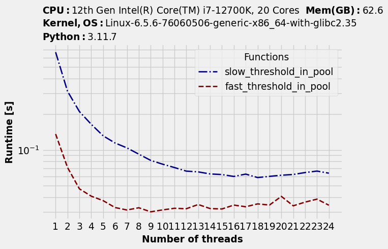
Notice how the run time declines as the number of threads increases… up to a point. After that run time starts getting worse again. So far this is what we’ve expected. But there is something unexpected too: the optimal number of threads is different for each function.
timings.to_dataframe().idxmin(axis="rows")
| Functions | Optimal number of threads |
|---|---|
| slow_threshold | 19 |
| fast_threshold | 9 |
The optimal level of parallelism also depends on your code
Our slower function was able to take advantage of basically all the logical cores. Possibly a single thread isn’t fully utilizing all the available processing in a given physical core, so logical cores allow for more parallelism.
In contrast, our faster function could take advantage of no more than 9 cores; beyond that it started slowing down. Perhaps it started hitting some bottleneck other than computation, like memory bandwidth.
There is no thread pool size that is optimal for both functions.
A different approach: empirical measurement
We’ve encountered multiple problems in getting the optimal number of threads:
- It’s difficult to get an accurate number of cores that take into account all the different ways the operating system can restrict CPU usage.
- The optimal parallelism level, e.g. number of threads, is workload dependent.
- The number of cores isn’t the only bottleneck.
- Bonus problem: If you’re running in the cloud, you’re using “vCPUs”, whatever that means. Different instances may have different CPU models, for one thing.
So here’s another approach: empirically discover the optimal number of threads, at runtime. In the example above we measured the optimal number of threads for a particular piece of code. If you have a long-running data processing job that will be running the same code for a while in multiple threads, you can do the same. That is, you can spend a little bit of time at the beginning to empirically measure the optimal number of threads, perhaps with some heuristics to compensate for noise.
For runtime purposes, if you’re using empirical measurement you don’t need to care about why a particular number of threads is optimal. Regardless of the hardware, operating system configuration, or cloud environment, you will be using the optimal level of parallelism.