From chunking to parallelism: faster Pandas with Dask
When data doesn’t fit in memory, you can use chunking: loading and then processing it in chunks, so that only a subset of the data needs to be in memory at any given time. But while chunking saves memory, it doesn’t address the other problem with large amounts of data: computation can also become a bottleneck.
How can you speed processing up?
One approach is to utilize multiple CPUs: pretty much every computer these days has more than one CPU. If you have two CPUs, you can often run your code (almost) twice as fast; four CPUs and you might approach a 4× speedup, and so on.
Even better, the chunking technique that helps reduce memory can also enable parallelism. Let’s see why, and then learn how the Dask library can easily enable parallelism of your Pandas processing code.
A quick recap: chunking
In a previous article I discussed how loading data in chunks can shrink memory use, and demonstrated how to structure code using the MapReduce pattern.
In this example we’re trying to figure out how many registered voters for each party live on each street in a city:
import pandas
from functools import reduce

# 1. Load. Read the data in chunks of 40000 records at a
#    time.
chunks = pandas.read_csv(
    "voters.csv", chunksize=40000, usecols=[
        "Residential Address Street Name ",
        "Party Affiliation "
    ]
)

# 2. Map. For each chunk, calculate the per-street counts:
def get_counts(chunk):
    by_party = chunk.groupby("Party Affiliation ")
    street = by_party["Residential Address Street Name "]
    return street.value_counts()
processed_chunks = map(get_counts, chunks)

# 3. Reduce. Combine the per-chunk voter counts:
def add(previous_result, new_result):
    return previous_result.add(new_result, fill_value=0)
result = reduce(add, processed_chunks)

# 4. Post-process.
result.sort_values(ascending=False, inplace=True)

print(result)
A key requirement for being able to process data in chunks is that the function we run on each chunk can run independently. In the example above, we can figure out how many voters are registered per-street in each chunk without reference to any of the other chunks.
If we can process chunks independently, that means we can process multiple chunks in parallel.
By utilizing our computer’s multiple CPUs, we can run the computation faster!
A little thought will suggest that the reduce step of adding together calculated counts is also, up to a point, independent enough to be run in parallel: A + B + C + D = (A + B) + (C + D).
So how can you implement parallelism with at little work as possible?
Dask: a parallel processing library
One of the easiest ways to do this in a scalable way is with Dask, a flexible parallel computing library for Python. Among many other features, Dask provides an API that emulates Pandas, while implementing chunking and parallelization transparently.
Because Dask is doing all the hard work for you, a good starting point is actually a more naive version of our task. Specifically, instead of implementing chunking, we’ll switch to Pandas code that loads all the data into memory at once:
import pandas

df = pandas.read_csv(
    "voters.csv", usecols=[
        "Residential Address Street Name ",
        "Party Affiliation "
    ]
)

def get_counts(df):
    by_party = df.groupby("Party Affiliation ")
    street = by_party["Residential Address Street Name "]
    return street.value_counts()

result = get_counts(df)
result.sort_values(ascending=False, inplace=True)

print(result)
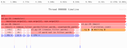
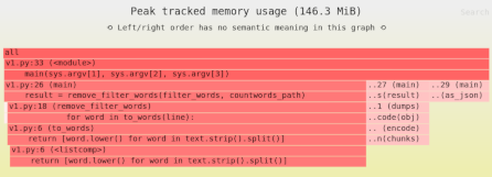
This is of course not ideal: it’s using only one CPU, and we need to load all the data into memory at once. Here’s what peak memory usage looks like:
Using Dask to emulate Pandas
The way Dask works involves two steps:
- First, you setup a computation, internally represented as a graph of operations.
- Then, you actually run the computation on that graph.
When Dask emulates the Pandas API, it doesn’t actually calculate anything; instead, it’s remembering what operations you want to do as part of the first step above.
Only once you run compute() does the actual work happen.
The result is code that looks quite similar, but behind the scenes is able to chunk and parallelize the implementation.
Here’s how we’d do this calculation with Dask:
import dask.dataframe as dd

# Load the data with Dask instead of Pandas.
df = dd.read_csv(
    "voters.csv",
    blocksize=16 * 1024 * 1024, # 16MB chunks
    usecols=["Residential Address Street Name ",
             "Party Affiliation "],
)

# Setup the calculation graph; unlike Pandas code,
# no work is done at this point:
def get_counts(df):
    by_party = df.groupby("Party Affiliation ")
    street = by_party["Residential Address Street Name "]
    return street.value_counts()
result = get_counts(df)

# Actually run the computation, using 2 threads:
result = result.compute(num_workers=2)

# Sort using normal Pandas DataFrame, since Dask's
# Pandas emulation doesn't implement this method:
result.sort_values(ascending=False, inplace=True)

print(result)
Notice that most of the code is unchaged! But as we’ll see execution time was faster, and memory usage is lower as well:
Note: Whether or not any particular tool or technique will speed things up depends on where the bottlenecks are in your software.
Need to identify the performance and memory bottlenecks in your own Python data processing code? Try the Sciagraph profiler, with support for profiling both in development and production on macOS and Linux, and with built-in Jupyter support.
Dask (usually) makes things better
The naive read-all-the-data Pandas code and the Dask code are quite similar. So how do they compare on memory usage and runtime, and to the original version which used chunks but wasn’t multi-threaded?
| Peak memory use | Wallclock time | CPU time | |
|---|---|---|---|
| Pandas (chunked) | 26 MiB | 5.9 seconds | 6.1 seconds |
| Pandas (naive) | 334 MiB | 6.7 seconds | 6.9 seconds |
| Dask | 88 MiB | 3.9 seconds | 6.5 seconds |
(If you don’t know the difference between wallclock and CPU time, see this article for details).
- In general, the naive version does the worst, both on memory usage and CPU time. CPU time may be slightly worse because the algorithms it uses don’t work well on really large chunks of data: both the chunked and Dask version are operating on smaller chunks of data at time.
- The chunked version uses the least memory, but wallclock time isn’t much better.
- The Dask version uses far less memory than the naive version, and finishes fastest (assuming you have CPUs to spare).
Dask isn’t a panacea, of course:
- Parallelism has overhead, it won’t always make things finish faster. And it doesn’t reduce the CPU time, so if you’re already saturating your CPUs it won’t speed things up on wallclock time either.
- Some tuning is needed. Larger block sizes increase memory use, but up to a point also allow faster processing.
If your task is simple or fast enough, single-threaded normal Pandas may well be faster.
For slow tasks operating on large amounts of data, you should definitely try Dask out. As you can see, it may only require very minimal changes to your existing Pandas code to get faster code with lower memory use.


