Let’s optimize! Running 15× faster with a situation-specific algorithm
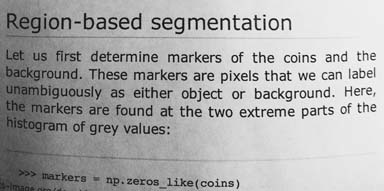
Let’s speed up some software! Our motivation: we have an image, a photo of some text from a book. We want to turn it into a 1-bit image, with just black and white, extracting the text so we can easily read it.
We’ll use an example image from scikit-image, an excellent image processing library:
from skimage.data import page
import numpy as np
IMAGE = page()
assert IMAGE.dtype == np.uint8
Here’s what it looks like (it’s licensed under this license):

Median-based local thresholding
The task we’re trying to do—turning darker areas into black, and lighter areas into white—is called thresholding. Since the image is different in different regions, with some darker and some lighter, we’ll get the best results if we use local thresholding, where the threshold is calculated from the pixel’s neighborhood.
Simplifying somewhat, for each pixel in the image we will:
- Calculate the median of the surrounding neighborhood.
- Subtract a magic constant from the calculated median to calculate our local threshold.
- If the pixel’s value is bigger than the threshold, the result is white, otherwise it’s black.
scikit-image includes an implementation of this algorithm. Here’s how we use it:
from skimage.filters import threshold_local

def skimage_median_local_threshold(img, neighborhood_size, offset):
    threshold = threshold_local(
        img, block_size=neighborhood_size, method="median", offset=offset
    )
    result = (img > threshold).astype(np.uint8)
    result *= 255
    return result

# The neighborhood size and offset value were determined "empirically", i.e.
# they're manually tuning the algorithm to work well with our specific
# example image.
SKIMAGE_RESULT = skimage_median_local_threshold(IMAGE, 11, 10)
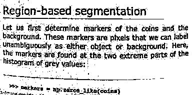
And here’s what the results look like:

Let’s see if we can make this faster!
Step 1. Reimplement our own version
We’re going to be using the Numba compiler, which lets us compile Python code to machine code at runtime. Here’s an initial implementation of the algorithm; it’s not quite identical to the original, for example the way edge pixels are handled, but it’s close enough for our purposes:
from numba import jit

@jit
def median_local_threshold1(img, neighborhood_size, offset):
    # Neighborhood size must be an odd number:
    assert neighborhood_size % 2 == 1
    radius = (neighborhood_size - 1) // 2
    result = np.empty(img.shape, dtype=np.uint8)

    # For every pixel:
    for i in range(img.shape[0]):
        # Calculate the Y borders of the neighborhood:
        min_y = max(i - radius, 0)
        max_y = min(i + radius + 1, img.shape[0])
        for j in range(img.shape[1]):
            # Calculate the X borders of the neighborhood:
            min_x = max(j - radius, 0)
            max_x = min(j + radius + 1, img.shape[1])
            # Calculate the median:
            median = np.median(img[min_y:max_y, min_x:max_x])
            # Set the image to black or white, depending how it relates to
            # the threshold:
            if img[i, j] > median - offset:
                # White:
                result[i, j] = 255
            else:
                # Black:
                result[i, j] = 0
    return result

NUMBA_RESULT1 = median_local_threshold1(IMAGE, 11, 10)
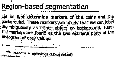
Here’s the resulting image; it looks similar enough that for our purposes:

Now we can compare the performance of the two implementations:
| Code | Elapsed milliseconds |
|---|---|
skimage_median_local_threshold(IMAGE, 11, 10) |
76 |
median_local_threshold1(IMAGE, 11, 10) |
87 |
It’s slower. But that’s OK, we’re just getting started.
Step 2: A faster implementation of the median algorithm
Calculating a median is pretty expensive, and we’re doing it for every single pixel, so let’s see if we can speed it up.
The generic median implementation Numba provides is likely to be fairly generic, since it needs to work in a wide variety of circumstances. We can hypothesize that it’s not optimized for our particular case. And even if it is, having our own implementation will allow for a second round of optimization, as we’ll see in the next step.
We’re going to implement a histogram-based median, based on the fact we’re using 8-bit images that only have a limited range of potential values. The median is the value where 50% of the pixels’ values are smaller, and 50% are bigger.
Here’s the basic algorithm for a histogram-based median:
- Each pixel’s value will go into a different bucket in the histogram; since we know our image is 8-bit, we only need 256 buckets.
- Then, we add up the size of each bucket in the histogram, from smallest to largest, until we hit 50% of the pixels we inspected.
@jit
def median_local_threshold2(img, neighborhood_size, offset):
    assert neighborhood_size % 2 == 1
    radius = (neighborhood_size - 1) // 2
    result = np.empty(img.shape, dtype=np.uint8)

    # 😎 A histogram with a bucket for each of the 8-bit values possible in
    # the image. We allocate this once and reuse it.
    histogram = np.empty((256,), dtype=np.uint32)

    for i in range(img.shape[0]):
        min_y = max(i - radius, 0)
        max_y = min(i + radius + 1, img.shape[0])
        for j in range(img.shape[1]):
            min_x = max(j - radius, 0)
            max_x = min(j + radius + 1, img.shape[1])

            # Reset the histogram to zero:
            histogram[:] = 0
            # Populate the histogram, counting how many of each value are in
            # the neighborhood we're inspecting:
            neighborhood = img[min_y:max_y, min_x:max_x].ravel()
            for k in range(len(neighborhood)):
                histogram[neighborhood[k]] += 1

            # Use the histogram to find the median; keep adding buckets until
            # we've hit 50% of the pixels. The corresponding bucket is the
            # median.
            half_neighborhood_size = len(neighborhood) // 2
            for l in range(256):
                half_neighborhood_size -= histogram[l]
                if half_neighborhood_size < 0:
                    break
            median = l

            if img[i, j] > median - offset:
                result[i, j] = 255
            else:
                result[i, j] = 0
    return result

NUMBA_RESULT2 = median_local_threshold2(IMAGE, 11, 10)
Here’s the resulting image:

And here’s the performance of our new implementation:
| Code | Elapsed milliseconds |
|---|---|
median_local_threshold1(IMAGE, 11, 10) |
86 |
median_local_threshold2(IMAGE, 11, 10) |
18 |
That’s better!
Step 3: Stop recalculating the histogram from scratch
Our algorithm uses a rolling neighborhood or window over the image, calculating the median for a window around each pixel. And the neighborhood for one pixel has a significant overlap for the neighborhood of the next pixel. For example, let’s say we’re looking at a neighborhood size of 3. We might calculate the median of this area:
......
.\\\..
.\\\..
.\\\..
......
......
And then when process the next pixel we’ll calculate the median of this area:
......
..///.
..///.
..///.
......
......
If we superimpose them, we can see there’s an overlap, the X:
......
.\XX/.
.\XX/.
.\XX/.
......
......
Given the histogram for the first pixel, if we remove the values marked
with \ and add the ones marked with /, we’ve calculated the exact
histogram for the second pixel. So for a 3×3 neighborhood, instead of
processing 3 columns we process 2, a minor improvement. For a 11×11
neighborhood, we will go from processing 11 columns to 2 columns, a much
more significant improvement.
Here’s what the code looks like:
@jit
def median_local_threshold3(img, neighborhood_size, offset):
    assert neighborhood_size % 2 == 1
    radius = (neighborhood_size - 1) // 2
    result = np.empty(img.shape, dtype=np.uint8)
    histogram = np.empty((256,), dtype=np.uint32)

    for i in range(img.shape[0]):
        min_y = max(i - radius, 0)
        max_y = min(i + radius + 1, img.shape[0])

        # Populate histogram as if we started one pixel to the left:
        histogram[:] = 0
        initial_neighborhood = img[min_y:max_y, 0:radius].ravel()
        for k in range(len(initial_neighborhood)):
            histogram[initial_neighborhood[k]] += 1

        for j in range(img.shape[1]):
            min_x = max(j - radius, 0)
            max_x = min(j + radius + 1, img.shape[1])

            # 😎 Instead of recalculating histogram from scratch, re-use the
            # previous pixel's histogram.

            # Substract left-most column we don't want anymore:
            if min_x > 0:
                for y in range(min_y, max_y):
                    histogram[img[y, min_x - 1]] -= 1

            # Add new right-most column:
            if max_x < img.shape[1]:
                for y in range(min_y, max_y):
                    histogram[img[y, max_x - 1]] += 1

            # Find the the median from the updated histogram:
            half_neighborhood_size = ((max_y - min_y) * (max_x - min_x)) // 2
            for l in range(256):
                half_neighborhood_size -= histogram[l]
                if half_neighborhood_size < 0:
                    break
            median = l
            if img[i, j] > median - offset:
                result[i, j] = 255
            else:
                result[i, j] = 0
    return result

NUMBA_RESULT3 = median_local_threshold3(IMAGE, 11, 10)
Here’s the resulting image:

And here’s the performance of our latest code:
| Code | Elapsed microseconds |
|---|---|
median_local_threshold2(IMAGE, 11, 10) |
17,066 |
median_local_threshold3(IMAGE, 11, 10) |
6,386 |
Step #4: Adapative heuristics
Notice that a median’s definition is symmetrical:
- The first value that is smaller than the highest 50% values.
- Or, the first value that is larger than the lowest 50% values. We used this definition in our code above, adding up buckets from the smallest to the largest.
Depending on the distribution of values, one approach to adding up buckets to find the median may be faster than the other. For example, given a 0-255 range, if the median is going to be 10 we want to start from the smallest bucket to minimize additions. But if the median is going to be 200, we want to start from the largest bucket.
So which side we should start from? One reasonable heuristic is to look at the previous median we calculated, which most of the time will be quite similar to the new median. If the previous median was small, start from the smallest buckets; if it was large, start from the largest buckets.
@jit
def median_local_threshold4(img, neighborhood_size, offset):
    assert neighborhood_size % 2 == 1
    radius = (neighborhood_size - 1) // 2
    result = np.empty(img.shape, dtype=np.uint8)
    histogram = np.empty((256,), dtype=np.uint32)
    median = 0

    for i in range(img.shape[0]):
        min_y = max(i - radius, 0)
        max_y = min(i + radius + 1, img.shape[0])

        histogram[:] = 0
        initial_neighborhood = img[min_y:max_y, 0:radius].ravel()
        for k in range(len(initial_neighborhood)):
            histogram[initial_neighborhood[k]] += 1

        for j in range(img.shape[1]):
            min_x = max(j - radius, 0)
            max_x = min(j + radius + 1, img.shape[1])

            if min_x > 0:
                for y in range(min_y, max_y):
                    histogram[img[y, min_x - 1]] -= 1

            if max_x < img.shape[1]:
                for y in range(min_y, max_y):
                    histogram[img[y, max_x - 1]] += 1

            half_neighborhood_size = ((max_y - min_y) * (max_x - min_x)) // 2
            # 😎 Find the the median from the updated histogram, choosing
            # the starting side based on the previous median; we can go from
            # the leftmost bucket to the rightmost bucket, or in reverse:
            the_range = range(256) if median < 127 else range(255, -1, -1)
            for l in the_range:
                half_neighborhood_size -= histogram[l]
                if half_neighborhood_size < 0:
                    median = l
                    break

            if img[i, j] > median - offset:
                result[i, j] = 255
            else:
                result[i, j] = 0
    return result

NUMBA_RESULT4 = median_local_threshold4(IMAGE, 11, 10)

The end result is 25% faster. Since the heuristic is tied to the image contents, the performance impact will depend on the image.
| Code | Elapsed microseconds |
|---|---|
median_local_threshold3(IMAGE, 11, 10) |
6,381 |
median_local_threshold4(IMAGE, 11, 10) |
4,920 |
The big picture
Here’s a performance comparison of all the versions of the code:
| Code | Elapsed microseconds |
|---|---|
skimage_median_local_threshold(IMAGE, 11, 10) |
76,213 |
median_local_threshold1(IMAGE, 11, 10) |
86,494 |
median_local_threshold2(IMAGE, 11, 10) |
17,145 |
median_local_threshold3(IMAGE, 11, 10) |
6,398 |
median_local_threshold4(IMAGE, 11, 10) |
4,925 |
Let’s go over the steps we went through:
- Switch to a compiled language: this gives us more control.
- Reimplement the algorithm taking advantage of constrained
requirements: our median only needed to handle
uint8, so a histogram was a reasonable solution. - Reuse previous calculations to prevent repetition: our histogram for the neighborhood of a pixel is quite similar to that of the previous pixel. This means we can reuse some of the calculations.
- Adaptively tweak the algorithm at runtime: as we run on an actual image, we use what we’ve learned up to this point to hopefully run faster later on. The decision from which side of the histogram to start is arbirary in general. But in this specific algorithm, the overlapping pixel neighborhoods mean we can make a reasonable guess.
This process demonstrates part of why generic libraries may be slower than custom code you write for your particular use case and your particular data.
Next steps
What else can you do to speed up this algorithm? Here are some ideas:
- There may be a faster alternative to histogram-based medians.
- We’re not fully taking advantage of histogram overlap; there’s also overlap between rows.
- The cumulative sum in the histogram doesn’t benefit from instruction-level parallelism or SIMD. It’s possible that using one of those would result in faster results even if it uses more instructions.
- So far the code has only used a single CPU. Given each row is calculated independently, parallelism would probably work well if done in horizontal stripes, probably taller than one pixel so as to maximize utilization of memory caches.
Want to learn more about optimizing compiled code for Python data processing? This article is an extract from a book I’m working on; test readers are currently going through initial drafts. Aimed at Python developers, data scientists, and scientists, the book covers topics like instruction-level parallelism, memory caches, and other performance optimization techniques. Learn more and sign up to get updates here.