Find slow data processing tasks (before your customers do)

Here are some of the ways you can discover your data processing jobs are too slow:

1. Jobs start getting killed when they hit timeouts.
2. Customers start complaining about slow or failed jobs.
3. Your cloud computing bill is twice what it was last month.

While these notification mechanisms do work, it’s probably best not to rely on them. Life is easier when jobs finish successfully, customers are happy, and you have plenty of money left over in your budget.

That means you want to identify unexpected slowness or high memory usage before the situation get that bad. The sooner you can identify performance problems, the sooner you can fix them.

So how can you identify inefficient tasks in your data pipeline or workflow? Let’s find out!

From “always slow” to “sometimes slow”

We’ll be focusing on data processing tasks, often running as part of a larger workflow or pipeline; this includes data science, scientific computing, and data analysis. Each job’s runtime has a particular structure:

1. Load some data as the input.
2. Process or analyze the input in some way, creating an output.
3. Store the resulting output, after which the job or task is finished.

When you first start implementing these sort of long-running tasks, you can reasonably assume that your code is inefficient. So to begin with, you can profile jobs at random, ideally in production, and use the profiling results to identify places where your code is too slow, or using too much memory. You fix the bottlenecks, measure again, and iterate until eventually you’ve created a sufficiently efficient baseline.

This is where the situation get more complex.

At this point most jobs are fast, but occasionally they’re slow. Perhaps because of environmental reasons, perhaps because different inputs give different behavior. Whatever the cause, the first step to fixing the underlying problem is identifying the specific jobs that are outliers: the jobs that are running more slowly than expected.

How do you identify these slow outliers? One approach is to use logging, something you probably want to do anyway to help with debugging and diagnostics.

Modeling performance and identifying outliers with logging

We can use logging to fix performance problems using a four step process:

1. Add logging to your program, ideally tracing-based logging.
2. Use logged information to build a model of your jobs’ speed.
3. The model can then help you identify outliers.
4. Inspect the outliers to identify and fix the problem.

Step 1. Add logging, which is necessary but not sufficient

To see how logging can be useful in identifying excessively slow tasks, I’m going to use trace-based logging, tracing for short, a superior form of logging. Specifically I’ll be using the OpenTelemetry standard, supported by many services and tools, and I’ll use the Honeycomb observability platform to visualize the data where possible. In practice you can use other services and/or normal logging and still get similar results, with differing degrees of difficulty.

Note: Honeycomb is pretty nice, but this use case is not its main focus. If you have suggestions for tracing observability services that are better designed for data processing jobs, let me know!

Let’s start with an example, a program that loads in a text file, filters out some words we don’t care about, and then writes out the words to a JSON file:

import sys
import json

def to_words(text):
    return [word.lower() for word in text.strip().split()]

def load_filter_words(filterwords_path):
    with open(filterwords_path) as f:
        return to_words(f.read())

def remove_filter_words(filter_words, countwords_path):
    result = []
    with open(countwords_path) as f:
        for line in f:
            for word in to_words(line):
                if word not in filter_words:
                    result.append(word)
    return result

def main(filterwords_path, countwords_path, output_path):
    filter_words = load_filter_words(filterwords_path)
    result = remove_filter_words(
        filter_words, countwords_path
    )
    with open(output_path, "w") as f:
        json.dump(result, f)

if __name__ == "__main__":
    main(sys.argv[1], sys.argv[2], sys.argv[3])

Next, let’s add some tracing with OpenTelemetry. Unlike normal logging which is a series of isolated events, OpenTelemetry traces execution using spans which have a beginning and end. Spans can have child spans, forming a tree of spans, and spans can have attached attributes. In the OpenTelemetry API, spans can be added using decorators, or with context managers:

@tracer.start_as_current_span("myspan")
def f():
    # ...

def g():
    with tracer.start_as_current_span("myspan2"):
        # ...

Each span is automatically nested within a parent span if it’s called inside its context.

In the following example, notice how the different steps of the task—loading, processing, and outputting data—each get their own span. We also make sure to record the input file size and the number of filter words as attributes.

# ...
from opentelemetry import trace
from opentelemetry.exporter.otlp.proto.http.trace_exporter import (
    OTLPSpanExporter,
)
from opentelemetry.sdk.trace import TracerProvider
from opentelemetry.sdk.trace.export import BatchSpanProcessor

TRACER = trace.get_tracer("example")

# ...
@TRACER.start_as_current_span("load_data")
def load_filter_words(filterwords_path):
    # ...

@TRACER.start_as_current_span("process_data")
def remove_filter_words(filter_words, countwords_path):
    # ...

def main(filterwords_path, countwords_path, output_path):
    # Initialize tracing:
    provider = TracerProvider()
    processor = BatchSpanProcessor(OTLPSpanExporter())
    provider.add_span_processor(processor)
    trace.set_tracer_provider(provider)

    with TRACER.start_as_current_span("main") as span:
        span.set_attribute(
            "input_size", os.path.getsize(countwords_path)
        )

        filter_words = load_filter_words(filterwords_path)
        span.set_attribute(
            "filter_words_count", len(filter_words)
        )

        result = remove_filter_words(
            filter_words, countwords_path
        )

        with TRACER.start_as_current_span("output_data"):
            with open(output_path, "w") as f:
                json.dump(result, f)

# ...

Now we can set a few environment variables, and when we run the task the trace info will get sent to Honeycomb:

$ python v2-with-tracing.py short-filter.txt middlemarch.txt output.json

Here’s an example of the resulting tree of spans for a single run, shown in the Honeycomb UI; we can see that in this example processing the data took the bulk of the time, followed by loading the data:

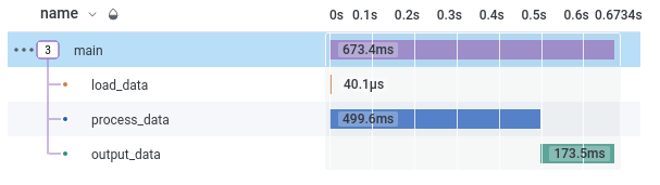
For each span, we have a number of attributes; those we explicitly recorded, but also some standard ones, including how long the span took to run: duration_ms. By doing a query on HEATMAP(duration_ms) for spans whose name is "main" (i.e. the top-level span), we can see that different tasks took different amounts of time (the Y axis). The X axis is when the task started.

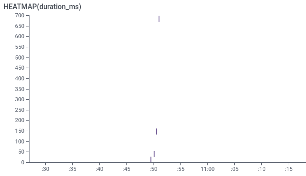
Since we want to find slow outliers, we want to focus on those tasks that are higher on the Y axis. For example, there’s a task took 700ms, compared to the much faster tasks below which only took up to 150ms. But is this 700ms task really an outlier?

The difficulty is that the run time is partially determined by input size. In our example, as is often the case, the larger input size, the longer the run time. If you have a smaller input, the task will run faster.

Here’s AVG(duration_ms) for "main" spans, grouped by input size; you can see that the larger the input size, the longer the span’s duration:

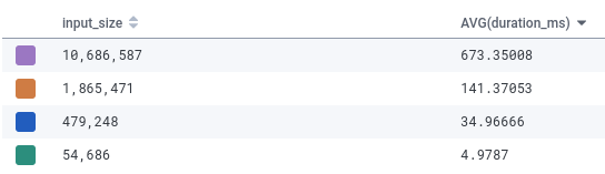
Sometimes you might consider that these slower tasks still count as outliers, in which case you can move on to step 4, fixing the problem. But running more slowly on larger output is often expected, normal behavior. That means you want a way to find outliers that takes the input size into account.

Step 2. Modeling expected run time based on input size

Since we’re logging input size, we can come up with a simplistic model:

1. The more words in our text document, the longer we expect it to run.
2. We’re logging file size, which isn’t quite the same as number of words, but is highly correlated.
3. It seems likely, both from our understanding of the code and from eyeballing the table above, that run time will be linear with number of words or file size.
4. Therefore, we expect duration_ms / input_size to be fairly constant; anything with a much higher ratio is an outlier.

Honeycomb allows you add “Derived Columns”, basically calculating a new attribute from existing attributes. In this case, we can add a column called duration_to_input, defined as DIV($duration_ms, $input_size).

Now if we build a table comparing AVG(duration_to_input) against input_size:

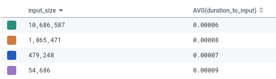
At this point input size is not the reason duration_to_input varies, and the range of values is much smaller: the biggest value is only 1.5× the smallest value, whereas previously we were seeing two orders of magnitude of range. So this seems like a reasonable model of performance; not perfect, but that’s OK.

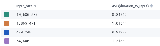
Since tiny numbers are harder to read, we can try to normalize them a bit, by dividing by the average value of 0.000075. We’ll change the formula to duration_ms / (input_size * 0.000075), or DIV($duration_ms, MUL($INPUT_SIZE, 0.000075)) in Honeycomb’s system.

Note: If you want to do this a bit more systemically, you can use SciPy to build a more mathematically accurate model. To get the raw data, Honeycomb lets you download query results as CSV.

Step 3. Identifying outliers

At this point we can say that if duration_to_input is around 0.7-1.3, we’re dealing with a normal result. If the values gets significantly higher, let’s say 1.5 or higher, we can consider than an outlier.

Let’s look at an example.

$ python v2-with-tracing.py long-filter.txt romanempire.txt output.json

If we look at Honeycomb, specifically at AVG(duration_to_input) grouped by trace.trace_id, so we can see individual runs, we see that this run is much slower. And critically, it’s much slower even after adjusting for input size:

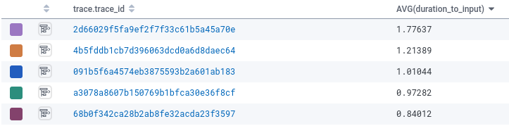
The new run had a ratio of 1.77, far above any other job. We’ve found an outlier!

Of course, manual queries aren’t the best way to find outliers. Once you’re comfortable with the model and have a sense of what a normal range is, you probably want to be automatically notified whenever outliers occur. Honeycomb has a feature called “Triggers” that will notify you when certain criteria are met; other tools should have similar functionality.

Step 4. Fixing bugs found via outliers and/or adjusting the model

A bit more investigation using Honeycomb’s UI (using the BubbleUp tool to compare outliers to baseline, or just reading the trace attributes) shows that this outlier has a different number of words to filter out. Previously we were using 30 words (short-filter.txt), this time we used 174 words (long-filter.txt).

It seems that performance is tied not just to number of words in the text document being filtered, as we first assumed, but also to the number of filter words.

Is this a performance bug, or should we just adjust our model to take into account the number of filter words? In this case, it’s probably a bug. Checking whether a string is contained in a set of other strings should be a fast, fairly constant O(1) operation if we were using a dictionary or set.

And that suggests the cause of the bug: we’re using a list for filter_words, so every word lookup is O(N) instead of O(1). That’s easy to fix, and while I won’t show that here, the result is that everything starts running faster.

Once we implement the fix, all the jobs will run faster, so we will need to tweak the duration_to_input model. But rather than making the model more complex, we just need to tweak it with a different constant, to take into account the faster baseline performance.

In other cases the fix may be less systemic, and the same performance model can continue unchanged.

Diagnosing performance problems with profiling

In this case, the code is short enough that the source code plus tracing info is sufficient to identify the problem. In real world code, it’s often far more difficult. This is where profiling comes in handy, as a complement to the information you get from logging: you really want to have profiling on by default in production.

Given continuous profiling in production, whenever you identify a slow identifier you will have immediate access to profiling information. For example, the Sciagraph performance profiler is designed specifically for Python data processing tasks, in both development and production. Here’s what it shows for this run:

It points you directly at if word not in filter_words: as the line where most of the time is spent.

Identifying memory usage outliers

So far we’ve been modeling performance runtime. But you might also want to identify jobs that are using too much memory, which can result in swapping, or being killed by the Linux out-of-memory killer. And that means customer complaints, failed jobs, and potentially high cloud costs.

To support finding outliers with high memory usage, we basically follow the exact same process, except that instead of using duration_ms or some other measure of elapsed time, we need to use a measure of memory usage. There are two basic ways you can measure memory, but either way we want peak memory, since that is the bottleneck in terms of hardware resources.

Option 1: Peak resident memory (RSS)

Peak resident memory is obtainable use the Python resource module; you can then add it as an attribute to the top-level span:

from resource import getrusage, RUSAGE_SELF

with TRACER.start_as_current_span("main"):
    # ...
    max_rss = getrusage(RUSAGE_SELF).ru_maxrss
    span.add_attribute("max_rss", max_rss)

However, as explained in more detail elsewhere, this measure is limited by available RAM, and can’t get higher. If you only have 8GB of RAM on your machine, you will never see more than 8GB; a program trying to allocate 8GB, 16GB or 32GB will report the same max resident memory, which can be misleading.

Option 2: Peak allocated memory

Alternatively, you can measure the peak amount of memory requested by the program. This also has issues, for example mmap() is only allocated lazily and so it’s unclear whether it should be counted or not until its dirty. On the other hand, this will tell you how much the program actually asked for, regardless of available RAM.

In addition to performance profiling, Sciagraph will also profile your job’s allocated memory usage, in production. And it comes with an OpenTelemetry integration that ensures the the peak allocated memory size also gets recorded in your logging/tracing system.

Alternatively, if you’re doing offline profiling you can use Fil or Memray for allocated memory profiling, but they’re not designed to be on-by-default in production.

You need logging!

As we said at the start of the article, you want happy customers, and plenty of money left in your bank account. This requires you to have sufficiently fast jobs. When you’re just starting out with some new code, you can simply:

1. Profile the code, ideally in production. No need to find outliers, just pick a job at random.
2. Identify the bottlenecks.
3. Fix the slowness.

Eventually, however, the normal case will be fast enough, and you will want to identify slow identifiers. This is where logging become useful; you probably already have some sort of logging already, for debugging purposes. You can also use logging to record the run time performance of you jobs, and build on that to identify slow outliers.

You don’t need to use Honeycomb to do so, nor do you need to use OpenTelemetry. I do hope someday there will be logging services designed specifically for larger scale batch jobs and data pipelines (and if they do exist, please tell me!). But even with Python’s built-in logging, logging a message at the end of the run with the elapsed time and input size is really very easy.

The important thing is that is to have some way to query the resulting logs and extract appropriate records. You’ll also want some way to get automatic notification of outliers. Then, whenever you identify outliers, you can look at your logs, look at your profiling, and immediately start fixing performance and memory problems—with any luck, before your customers notice.